Structured Prediction Exercises - Solutions
Contents
$$ \newcommand{\Xs}{\mathcal{X}} \newcommand{\Ys}{\mathcal{Y}} \newcommand{\y}{\mathbf{y}} \newcommand{\repr}{\mathbf{f}} \newcommand{\repry}{\mathbf{g}} \newcommand{\x}{\mathbf{x}} \newcommand{\vocab}{V} \newcommand{\params}{\boldsymbol{\theta}} \newcommand{\param}{\theta} \DeclareMathOperator{\perplexity}{PP} \DeclareMathOperator{\argmax}{argmax} \DeclareMathOperator{\argmin}{argmin} \newcommand{\train}{\mathcal{D}} \newcommand{\counts}[2]{#_{#1}(#2) } \newcommand{\indi}{\mathbb{I}} $$
Structured Prediction Exercises - Solutions#
Setup 1: Load Libraries#
%%capture
%load_ext autoreload
%autoreload 2
%matplotlib inline
import sys
sys.path.append("..")
import statnlpbook.util as util
import matplotlib
import matplotlib.pyplot as plt
matplotlib.rcParams['figure.figsize'] = (10.0, 6.0)
---------------------------------------------------------------------------
ModuleNotFoundError                       Traceback (most recent call last)
Input In [1], in <cell line: 6>()
      4 import sys
      5 sys.path.append("..")
----> 6 import statnlpbook.util as util
      7 import matplotlib
      8 import matplotlib.pyplot as plt

ModuleNotFoundError: No module named 'statnlpbook'
Task 1 solution#
We need to find a different representation and model that also achieves perfect accuracy.
There are several different ways you can represent your input and your output, for example:
length of a sentence in characters (as presented in lecture notes)
length of a sentence in words (presented solution)
number of empty spaces in a sentence, as a surrogate for a length in words (question: what might be a problem with this representation?)
ratio of English/German sentence lengths (question: what is a possible issue with this representation?)
…
def new_f(x):
    """Calculate a representation of the input `x`."""
    return len(x.split(' '))

def new_g(y):
    """Calculate a representation of the output `y`."""
    return len(y.split(' '))
As for the model, again, there are several different types of model one can think of:
negative absolute value of scaled English length and German length (as presented in lecture notes)
variations on the previous one, based on the position and effect of the parameter to any of the representations
negative of a square of differences (presented solution)
variations with ratios of representations instead of their difference (question: which problems might you expect with this model?) …
def new_s(theta,x,y):
    """Measure the compatibility of sentences `x` and `y` using parameter `theta`"""
    return -pow(theta * f(x) - g(y), 2)
Before going on to the next solution, run the following code to initialise the model and representations to the ones used in the lecture notes:
import math
import numpy as np

x_space = ['I ate an apple',
           'I ate a red apple',
           'Yesterday I ate a red apple',
           'Yesterday I ate a red apply with a friend']
y_space = ['Ich aß einen Apfel',
           'Ich aß einen roten Apfel',
           'Gestern aß ich einen roten Apfel',
           'Gestern aß ich einen roten Apfel mit einem Freund']
data = list(zip(x_space,y_space))
train = data[:2]
test = data[2:]

def f(x):
    """Calculate a representation of the input `x`."""
    return len(x)
def g(y):
    """Calculate a representation of the output `y`."""
    return len(y)

def s(theta,x,y):
    """Measure the compatibility of sentences `x` and `y` using parameter `theta`"""
    return -abs(theta * f(x) - g(y))

thetas = np.linspace(0.0, 2.0, num=1000)
Task 2 solution#
We need to find a “smoother” objective that is continuous and has optima that also optimase the original zero-one loss:
def zero_one_loss(theta, data):
    """Measure the total number of errors made when predicting with parameter `theta` on training set `data`"""
    total = 0.0
    for x,y in data:
        max_score = -math.inf
        result = None
        for y_guess in y_space:
            score = s(theta,x,y_guess)
            if score > max_score:
                result = y_guess
                max_score = score
        if result != y:
            total += 1.0
    return total

plt.plot(thetas, [zero_one_loss(theta,train) for theta in thetas])
---------------------------------------------------------------------------
NameError                                 Traceback (most recent call last)
Input In [5], in <cell line: 16>()
     13             total += 1.0
     14     return total
---> 16 plt.plot(thetas, [zero_one_loss(theta,train) for theta in thetas])

NameError: name 'plt' is not defined
Zero-one loss is a discrete loss, and we’d like to find a smoother one (question: why do we prefer smoother losses?). The problem of finding a smoother loss boils down to finding new types of loss which incorporate score information in loss calculation, specifically, some contrast between the score of a gold output structure $\y$ of $(\x,\y) \in \train$ and the score of the highest scoring German sentence $\y’{\param}=\argmax\y s_\param(\x,\y)$, or a combination of multiple scores for several output structures $\y \in \Ys$.
There are several different losses one might implement:
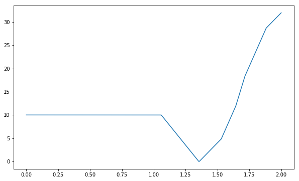
Structured perceptron loss#
$$ l(\param)=\sum_{(\x,\y) \in \train} (s_\param(\x,\y’{\param}) - s\param(\x,\y)) $$
def structured_perceptron_loss(theta, data):
    """Measure the total number of errors made when predicting with parameter `theta` on training set `data`"""
    total = 0.0
    for x,y in data:
        max_score = -math.inf
        result = None
        for y_guess in y_space:
            score = s(theta,x,y_guess)
            if score > max_score:
                result, max_score = y_guess, score
        # the loss (per instance) is a deviation of the score of the highest-scored instance from the score of the true label
        total += max_score - s(theta, x, y)
    return total

plt.plot(thetas, [structured_perceptron_loss(theta,train) for theta in thetas])
[<matplotlib.lines.Line2D at 0x10fe35b38>]
Structured perceptron hinge loss#
$$ l(\param)=\sum_{(\x,\y) \in \train} (\sum_{\y \in \Ys}(\max(0, s_\param(\x,\y’{\param}) - s\param(\x,\y) + \Delta))) $$
def hinge_loss(theta, data, delta=4.0):
    """Measure the total number of errors made when predicting with parameter `theta` on training set `data`"""
    total = 0.0
    for x,y in data:
        for y_guess in y_space:
            if y != y_guess:
                # per instance, whenever you make a mistake, add the max of zero and difference between score of every structured output increased by a margin (yet another parameter!)
                total += max(0, s(theta, x, y_guess) - s(theta, x, y) + delta)
    return total

plt.plot(thetas, [hinge_loss(theta,train) for theta in thetas])
[<matplotlib.lines.Line2D at 0x1101e6470>]
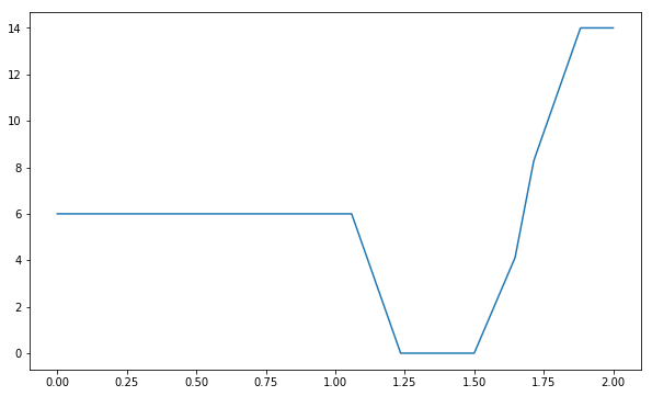
Log loss#
$$ l(\param)=\sum_{(\x,\y) \in \train} (log(\sum_{\y \in \Ys} e^{s_\param(\x,\y’{\param})}) - s\param(\x,\y)) $$
from math import exp, log
# cross entropy loss
def log_loss(theta, data):
    """Measure the total number of errors made when predicting with parameter `theta` on training set `data`"""
    total = 0.0
    for x,y in data:
        max_score = -math.inf
        sum_exp = 0.0
        for y_guess in y_space:
            sum_exp += exp(s(theta,x,y_guess))
        # this is a soft version of the max function called softmax
        # e to the power of score of the true output structure, divided by the sum of e to the power of score for all possible output structures
        total += -log(exp(s(theta, x, y)) / sum_exp)
    return total

plt.plot(thetas, [log_loss(theta,train) for theta in thetas])
[<matplotlib.lines.Line2D at 0x110354f28>]

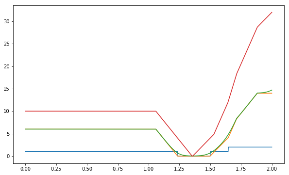
Loss comparison#
It’s useful to plot all the losses we define to visually compare them and verify that they all end up with minimum in the same interval.
plt.plot(thetas, [zero_one_loss(theta,train) for theta in thetas],
         thetas, [structured_perceptron_loss(theta,train) for theta in thetas],
         thetas, [log_loss(theta,train) for theta in thetas],
         thetas, [hinge_loss(theta,train) for theta in thetas]
        )
[<matplotlib.lines.Line2D at 0x1104da6a0>,
 <matplotlib.lines.Line2D at 0x1104dafd0>,
 <matplotlib.lines.Line2D at 0x1104e0898>,
 <matplotlib.lines.Line2D at 0x1104e0a58>]